
| 일 | 월 | 화 | 수 | 목 | 금 | 토 |
|---|---|---|---|---|---|---|
| 1 | 2 | 3 | 4 | 5 | 6 | |
| 7 | 8 | 9 | 10 | 11 | 12 | 13 |
| 14 | 15 | 16 | 17 | 18 | 19 | 20 |
| 21 | 22 | 23 | 24 | 25 | 26 | 27 |
| 28 | 29 | 30 | 31 |
- Computer Vision
- Semantic Segmentation
- 딥러닝
- 논문
- pytorch
- 머신러닝
- optimizer
- transformer
- 논문리뷰
- opencv
- ViT
- 파이썬
- Ai
- 파이토치
- object detection
- 인공지능
- 프로그래머스
- 코딩테스트
- Python
- Self-supervised
- 논문구현
- Segmentation
- 논문 리뷰
- 코드구현
- Paper Review
- cnn
- 옵티마이저
- 알고리즘
- Convolution
- programmers
- Today
- Total
Attention please
[논문 리뷰] Inception V1 - GoogLeNet(2014), 파이토치 구현 본문
[논문 리뷰] Inception V1 - GoogLeNet(2014), 파이토치 구현
Seongmin.C 2022. 12. 28. 02:02이번에 리뷰할 논문은 "Going deeper with convolutions" 이다. 이 논문에서 나온 이른바 GoogLeNet은 이미지넷 이미지 인식 대회(ILSVRC)에서 앞서 설명한 VGGNet을 이기고 우승을 차지한 모델이다. GoogLetNet은 VGG-19보다 더 깊은 22층으로 구성된 알고리즘이다.
GoogLeNet은 1 x 1 와 같이 작은 사이즈의 convolution 층을 사용했다는 점과 층을 깊게 쌓아 모델의 성능을 개선하려한 점에서 VGGNet과 유사한 점들이 많다. 하지만 GoogLeNet만의 독특한 점이 있었는데 바로 인셉션(Inception)이다.
Architecture
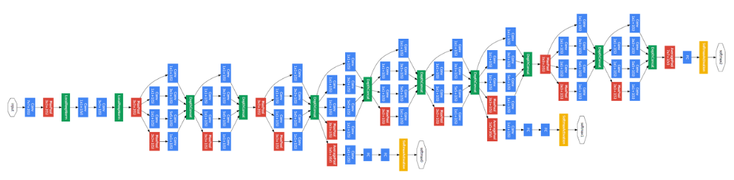
위 figure가 GoogLeNet의 구조이다. 앞서 말했던 것처럼 층이 총 22개 존재함을 볼 수 있다. GoogLeNet의 중요한 특징으로는 크게 3가지가 있는데 1x1 Convolution, Inception module, global average pooling 이다.
1 x 1 Convolution
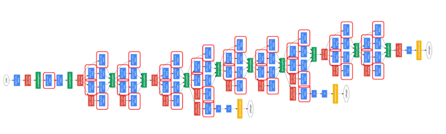
다음은 1x1 Conv에 해당하는 층을 표시해 놓은 것이다. 위 그림을 보면 1x1 Conv을 곳곳에 사용한 것을 볼 수 있다. 그렇다면 왜 1x1 Conv를 사용하는 것일까?
1x1 Conv를 사용하는 이유는 Feature map의 개수를 줄이기 위해서 사용된다. 또 feature map의 개수가 줄어들게 되면 연산량이 줄어들기 때문에 1x1 Conv를 사용하는 것이다.
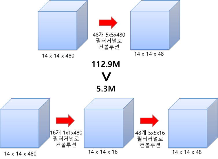
예를 들어, (14x14x480) 의 입력데이터가 들어와 바로 48개의 (5x5x480) 필터커널과 합성곱을 하게 되면 (14x14x48) 의 출력데이터가 나오게 된다. 이때 필요한 연산량은 (14x14x48) x (5x5x480) = 약 112.9M 이다.
이번에는 1x1 Conv를 사용해보자. 똑같이 (14x14x480) 의 입력데이터가 들어왔지만 전과 다르게 16개의 (1x1x480) 필터커널과 합성곱을 한 후 48개의 (5x5x16) 필터 커널과 합성곱을 하여 (14x14x48) 의 출력데이터가 나오게 된다. 이때 필요한 연산량은 (14x14x16) x (1x1x480) + (14x14x48) x (5x5x16) = 약 5.3M 이다.
1x1 Conv를 사용하지 않았을 때와 사용했을 때 출력값은 동일하지만 연산량은 1x1 Conv를 사용했을 때 확연히 줄어든 것을 확인할 수 있다. 연산량이 줄어들수록 모델의 층을 더 깊게 쌓을 수 있기 때문에 이는 모델의 성능을 높이는데 중요하다.
Inception Module
Inception 모듈은 GoogLeNet의 핵심이라 볼 수 있다. Inception에 대해 간단히 설명하자면 합성곱에 사용되는 feature map의 크기에 따라 서로 다른 level의 feature를 추출할 수 있다. 따라서 다양한 level의 feature를 효과적으로 추출하기 위해서 1x1, 3x3, 5x5 Conv를 병렬적으로 수행하는 것이 Inception 모듈이다.
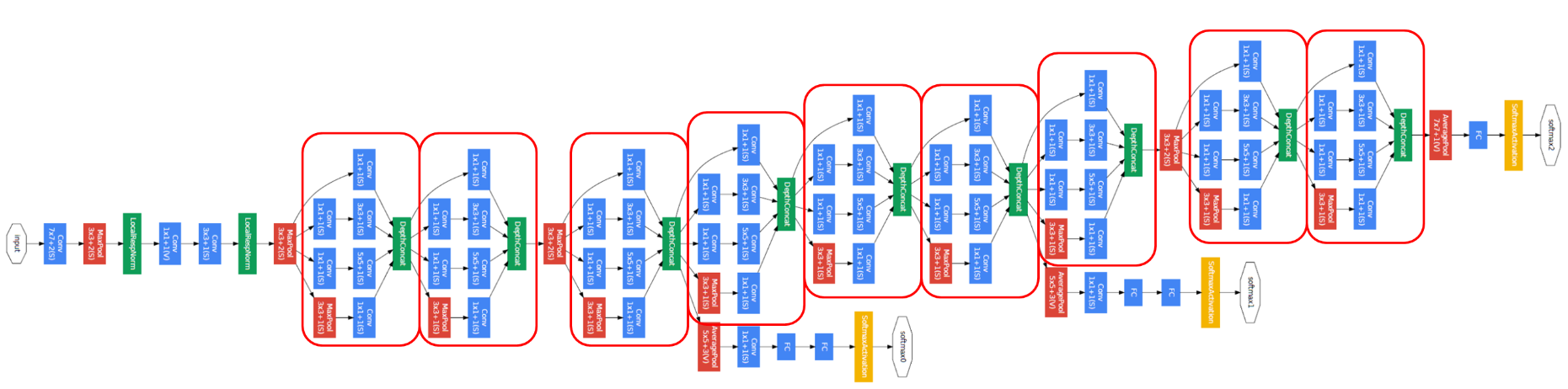
하지만 filter의 사이즈가 커지면 커질 수록 연산량은 점점 커지게 된다. 즉, 5x5 Conv를 사용하게되면 연산량이 증가한다는 문제가 있었는데 이를 해결하기 위해서 위에서 다룬 1x1 Conv를 사용한다.
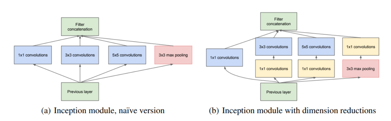
3x3 Conv 와 5x5 Conv 전에 1x1 Conv를 두어 연산량을 줄였고 이는 다양한 level의 feature를 추출하면서도 연산량을 줄여 모델의 성능을 높일 수 있었다.
Global Average Pooling
지금까지의 CNN모델이었던 AlexNet과 VGGNet에서는 후반부에 FC(Fully Connected) layer을 연결하였다. 즉 Conv층을 거치고 나온 데이터를 flatten을 시킨 후 가중치를 곱하여 분류를 하였는데 GoogLeNet에서는 FC 방식 대신 GAP(Global Average Pooling) 방식을 사용한다.
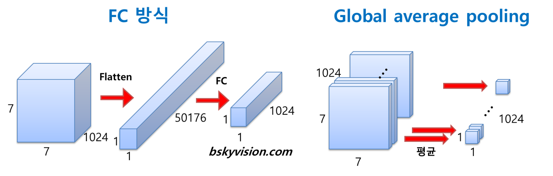
Conv층을 거쳐 나온 데이터를 flatten 시켜주는 FC 방식과는 다르게 GAP는 각 feature map에 대해 평균을 내준 후 그 값들을 이어 1차원 벡터를 만들어 준다.
GAP를 사용하게 되면 FC 방식을 사용했을 때보다 가중치의 개수가 줄어 연산량이 상당히 줄어든다.
Auxiliary Classifier
모델의 깊이가 늘어나면 성능이 높아진다는 장점이 있지만 같이 따라오는 단점들도 존재하는데 그 중 하나가 바로 vanishing gradient 문제이다. GoogLeNet은 이를 해결하기 위해 네트워크 중간에 보조 분류기를 달아주었다.

모델의 마지막 layer에만 softmax를 놓지 않고, 중간중간 추가적인 classifier를 추가함으로써 중간에서도 역전파가 진행되도록 한다. 물론 Auxiliary Classifier은 vanishing gradient 문제만을 해결하기 위해 사용하는 기법이기에 train할 때만 사용하고 test할 때는 제거해준 후 마지막 layer의 softmax만을 사용한다.
코드 구현
지금까지 알아본 GoogLeNet 모델을 파이토치를 사용하여 구현해보자.
GoogLeNet 모델에는 다양한 사이즈의 Conv층이 이어지는 경우가 빈번하다. 보다 편하게 구현하기 위해 Conv층이 이어지는 구간을 함수로 정의해주자.
# 1x1 Convolution
def conv_1(in_dim, out_dim):
    model = nn.Sequential(
        nn.Conv2d(in_dim, out_dim, kernel_size=1, stride=1),
        nn.BatchNorm2d(out_dim),
        nn.ReLU()
    )
    return model

# 1x1 Convolution -> 3x3 Convolution
def conv_1_3(in_dim, mid_dim, out_dim):
    model = nn.Sequential(
        nn.Conv2d(in_dim, mid_dim, 1, 1),
        nn.BatchNorm2d(mid_dim),
        nn.ReLU(),
        nn.Conv2d(mid_dim, out_dim, 3, 1, padding=1),
        nn.BatchNorm2d(out_dim),
        nn.ReLU()
    )
    return model

# 1x1 Convolution -> 5x5 Convolution
def conv_1_5(in_dim, mid_dim, out_dim):
    model = nn.Sequential(
        nn.Conv2d(in_dim, mid_dim, 1, 1),
        nn.BatchNorm2d(mid_dim),
        nn.ReLU(),
        nn.Conv2d(mid_dim, out_dim, 5, 1, padding=2),
        nn.BatchNorm2d(out_dim),
        nn.ReLU()
    )
    return model

# 3x3 MaxPooling -> 1x1 Convolution

def max_3_1(in_dim, out_dim):
    model = nn.Sequential(
        nn.MaxPool2d(kernel_size=3, stride=1, padding=1),
        nn.Conv2d(in_dim, out_dim, 1, 1),
        nn.BatchNorm2d(out_dim),
        nn.ReLU()
    )
    return model
다음으로는 GoogLeNet의 핵심인 Inception Module를 정의해보자. 위에서 미리 정의해놓은 함수들을 사용하여 concat을 해주기만 하면 된다.
class inception_module(nn.Module):
    def __init__(self, in_dim, out_dim_1, mid_dim_3, out_dim_3, mid_dim_5, out_dim_5, pool_dim):
        super(inception_module, self).__init__()
        # 1x1 Convolution
        self.conv_1 = conv_1(in_dim, out_dim_1)

        # 1x1 Convolution -> 3x3 Convolution
        self.conv_1_3 = conv_1_3(in_dim, mid_dim_3, out_dim_3)

        # 1x1 Convolution -> 5x5 Convolution
        self.conv_1_5 = conv_1_5(in_dim, mid_dim_5, out_dim_5)

        # 3x3 MaxPooling -> 1x1 Convolution
        self.max_3_1 = max_3_1(in_dim, pool_dim)

    def forward(self, x):
        out_1 = self.conv_1(x)
        out_2 = self.conv_1_3(x)
        out_3 = self.conv_1_5(x)
        out_4 = self.max_3_1(x)
        # concat
        output = torch.cat([out_1,out_2,out_3,out_4], dim=1)  # 가로 방향(dim=1)으로 합치기
        return output
이제 위에서 정의한 것들을 이용하여 GoogLeNet을 구현해보자. 각 층의 size와 채널 등등 파라미터 값들은 해당 논문과 동일하게 구현하였다.

class GoogLeNet(nn.Module):
    def __init__(self, base_dim=64, num_classes=10):
        super(GoogLeNet, self).__init__()
        self.num_classes=num_classes
        self.layer_1 = nn.Sequential(
            nn.Conv2d(3, base_dim, 7, 2, 3),
            nn.BatchNorm2d(base_dim),
            nn.MaxPool2d(3, 2, 1),
            nn.Conv2d(base_dim, base_dim*3, 3, 1, 1),
            nn.BatchNorm2d(base_dim*3),
            nn.MaxPool2d(3, 2, 1)
        )
        self.layer_2 = nn.Sequential(
            inception_module(base_dim*3, 64, 96, 128, 16, 32, 32),
            inception_module(base_dim*4, 128, 128, 192, 32, 96, 64),
            nn.MaxPool2d(3, 2, 1)
        )
        self.layer_3 = nn.Sequential(
            inception_module(480, 192, 96, 208, 16, 48, 64),
            inception_module(512, 160, 112, 224, 24, 64, 64),
            inception_module(512, 128, 128, 256, 24, 64, 64),
            inception_module(512, 112, 144, 288, 32, 64, 64),
            inception_module(528, 256, 160, 320, 32, 128, 128),
            nn.MaxPool2d(3,2,1)
        )
        self.layer_4 = nn.Sequential(
            inception_module(832, 256, 160, 320, 32, 128, 128),
            inception_module(832, 384, 192, 384, 48, 128, 128),
            nn.AvgPool2d(8, 1)
        )
        self.layer_5 = nn.Dropout2d(p=0.4)
        self.fc_layer = nn.Linear(1024, 10)

    def forward(self, x):
        out = self.layer_1(x)
        out = self.layer_2(out)
        out = self.layer_3(out)
        out = self.layer_4(out)
        out = self.layer_5(out)
        out = out.view(out.size(0), -1)
        out = self.fc_layer(out)
        return out


net = GoogLeNet().to(device)
print(net)
'논문 리뷰 > Image classification' 카테고리의 다른 글
| [논문 리뷰] DenseNet(2017), 파이토치 구현 (0) | 2022.12.29 |
|---|---|
| [논문 리뷰] Xception(2017), 파이토치 구현 (0) | 2022.12.29 |
| [논문 리뷰] ResNet(2016), 파이토치 구현 (0) | 2022.12.28 |
| [논문 리뷰] VGGNet(2015), 파이토치 구현 (0) | 2022.10.01 |
| [논문 리뷰] AlexNet(2012), 파이토치 구현 (0) | 2022.09.29 |


